Search Algorithms

A search algorithm tries to find whether a target value exists in a collection, or where that value is stored.

The key question is: what do we know about the data before searching?

Different search algorithms make different assumptions:

Algorithm	Data needed before search	Main idea	Worst-case time
linear search	data can be unsorted	check items one by one	$O(n)$
binary search	data must be sorted	repeatedly halve the possible range	$O(\log n)$
hash table search	data must be stored using a hash table	use the key to compute where to look	$O(n)$ worst case

Here, n means the number of items being searched. Big-O notation, such as $O(n)$ or $O(\log n)$, describes how the amount of work grows as n becomes larger. It is not an exact running time in seconds. For example, $O(n)$ means the work can grow roughly in proportion to the number of items, while $O(\log n)$ means the work grows much more slowly because the search space is repeatedly reduced. See Algorithm Efficiency and Tracing for the full explanation.

The aim is not only to know the final answer. You should be able to trace the state of the algorithm as it runs.

What the Return Value Means

Many search algorithms return an index.

• If the target is found, the algorithm returns the index where the target is stored.
• If the target is not found, the algorithm returns -1.

For example, if a search in [13, 8, 21, 5] returns 2, it means the target is stored at index 2. If it returns -1, it means the target is absent.

Some programs return True or False instead. That is also possible, but index-returning versions are useful because they tell us both whether the item exists and where it is found.

Linear Search

Linear search checks items one by one from the start until the target is found or the list ends.

It is the simplest search method because it makes no special assumption about the order of the data.

Use linear search when:

• the list is unsorted;
• the list is small;
• simplicity is more important than speed;
• the data is not stored in a structure that supports faster lookup.

Core Idea

Linear search asks the same question repeatedly:

Is this item equal to the target?

If yes, return the current index. If no, move to the next item.

If the loop finishes without finding the target, every item has been checked, so the algorithm returns -1.

Pseudocode

FUNCTION LinearSearch(items, target)
    FOR index <- 0 TO LENGTH(items) - 1
        IF items[index] = target THEN
            RETURN index
        ENDIF
    NEXT index
 
    RETURN -1
ENDFUNCTION

This pseudocode assumes zero-based indexing: the first item is at index 0, the second item is at index 1, and so on. If LENGTH(items) is the total number of items, then the last valid index is LENGTH(items) - 1. For example, a list of 4 items has indexes 0, 1, 2, and 3.

An equivalent WHILE-loop version initialises index <- 0, repeats while index < LENGTH(items), and increments index after each failed comparison. The algorithmic idea and $O(n)$ worst case are unchanged; only the loop construct differs.

Original Python Example

def linear_search(items, target):
    for index, item in enumerate(items):
        if item == target:
            return index
    return -1

Trace: Target Found

Trace for items = [13, 8, 21, 5], target = 21:

Step	index	item	comparison	result
1	0	13	13 == 21 is false	continue
2	1	8	8 == 21 is false	continue
3	2	21	21 == 21 is true	return 2

The search stops immediately when the target is found. The item at index 3 is not checked because the answer is already known.

Trace: Target Absent

Trace for items = [13, 8, 21, 5], target = 7:

Step	index	item	comparison	result
1	0	13	13 == 7 is false	continue
2	1	8	8 == 7 is false	continue
3	2	21	21 == 7 is false	continue
4	3	5	5 == 7 is false	continue
after loop	-	-	no items left	return -1

The absent case is important. It shows why the algorithm needs a final RETURN -1 after the loop.

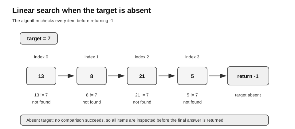
Caption: When the target is absent, every comparison fails, so linear search inspects all items before returning -1.

Linear Search Invariant

An invariant is something that remains true while an algorithm is running.

For linear search, after checking index i, all items from index 0 to index i are known not to be the target, unless the algorithm has already returned.

This is why the algorithm can safely move forward one item at a time.

Complexity of Linear Search

Linear search has worst-case time $O(n)$.

In the worst case:

• the target is the last item; or
• the target is absent.

In both cases, the algorithm may need to check all n items.

The best case is faster: if the target is at index 0, only one item is checked. However, the worst-case time is still $O(n)$ because the algorithm cannot assume that the target will be first.

Binary Search

Binary search works only on sorted data. It compares the target with the middle item, then discards the half where the target cannot be.

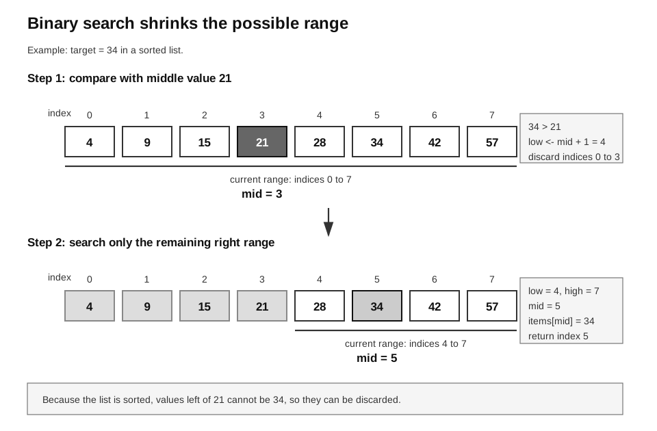
Caption: Read each row from the active low..high range to mid, then follow the highlighted surviving half. The discarded half is safe to remove only because the values are sorted; the remaining range must become strictly smaller after every unsuccessful comparison.

Why Sorted Data Is Required

Binary search depends on order.

Suppose the list is sorted in ascending order. If the target is larger than the middle value, then the target cannot be in the left half. Every value in the left half is less than or equal to the middle value.

This reasoning fails if the list is unsorted.

For a concrete failure, consider the unsorted list [10, 4, 8, 2] and target 10. With low = 0, high = 3, the lower middle index is 1, whose value is 4. The algorithm discards indexes 0..1 because 10 > 4, even though the target was at index 0. It eventually returns -1 incorrectly. The fault is not binary search itself; its sorted-input precondition was violated.

Core Idea

Binary search keeps a possible search range.

The main variables are:

Variable	Meaning
low	index of the first possible position
high	index of the last possible position
mid	index of the middle item in the current range

At each step:

1. Compute mid.
2. Compare items[mid] with the target.
3. If the target is found, return mid.
4. If the target is larger, move low to mid + 1.
5. If the target is smaller, move high to mid - 1.

The range becomes smaller after each comparison.

Loop invariant: if the target exists, it remains somewhere in the inclusive index range low..high. Each update must preserve this claim while making the range strictly smaller.

Pseudocode

FUNCTION BinarySearch(items, target)
    low <- 0
    high <- LENGTH(items) - 1
 
    WHILE low <= high
        mid <- (low + high) DIV 2
 
        IF items[mid] = target THEN
            RETURN mid
        ELSE IF target > items[mid] THEN
            low <- mid + 1
        ELSE
            high <- mid - 1
        ENDIF
    ENDWHILE
 
    RETURN -1
ENDFUNCTION

Original Python Example

def binary_search(items, target):
    low = 0
    high = len(items) - 1
 
    while low <= high:
        mid = (low + high) // 2
        if items[mid] == target:
            return mid
        if target > items[mid]:
            low = mid + 1
        else:
            high = mid - 1
 
    return -1

This implementation uses inclusive low and high bounds and the lower middle index (low + high) // 2. Other correct variants exist, but their loop condition and boundary updates must match their chosen bounds. With duplicate target values, this ordinary version returns a matching index, not necessarily the first or last occurrence.

Recursion bridge

Binary search can also be written recursively: compare the middle item, return on a match, otherwise call the procedure again with either low <- mid + 1 or high <- mid - 1. Its base case is low > high, which returns -1. This is the same halving strategy as the iterative version; it is included to connect this algorithm to recursion, not as a second core algorithm to memorise.

Trace: Target Found

Trace for items = [4, 9, 15, 21, 28, 34, 42, 57], target = 34:

In each row, low, high, and mid are positional indexes, not values from the list. For example, mid = 3 means “look at the item stored at index 3”. The value at that position is items[3] = 21.

The algorithm uses low and high to mark the current possible search range. It computes mid = (low + high) DIV 2, compares items[mid] with the target, then either finds the target or discards one half of the range.

Step	possible index range	mid calculation	middle value	comparison and action
1	low = 0, high = 7, so indexes 0..7 are possible	(0 + 7) DIV 2 = 3	items[3] = 21	34 > 21, so the target must be to the right; set low <- 4
2	low = 4, high = 7, so indexes 4..7 are possible	(4 + 7) DIV 2 = 5	items[5] = 34	34 = 34, so return index 5

Binary search does not check every item. It uses the sorted order to remove impossible positions.

Trace: Target Absent

Trace for items = [4, 9, 15, 21, 28, 34, 42, 57], target = 30:

Step	low	high	mid	middle value	action
1	0	7	3	21	target is larger, set low to 4
2	4	7	5	34	target is smaller, set high to 4
3	4	4	4	28	target is larger, set low to 5
after loop	5	4	-	-	low > high, return -1

The condition low > high means the possible search range is empty. There is no index left where the target could be.

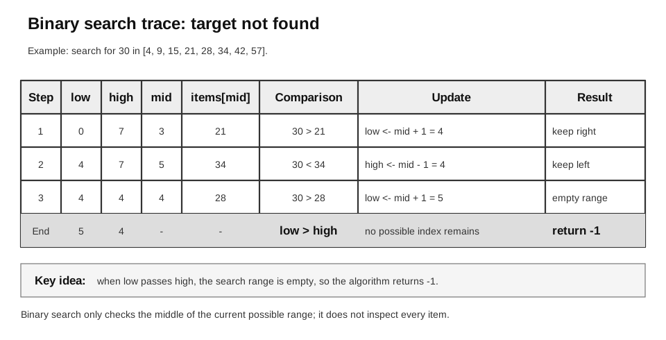
Caption: A not-found binary search updates low and high until low > high, meaning the search range is empty and the algorithm returns -1.

Why low <= high Is Used

The loop condition is usually low <= high because a range with one item left still needs to be checked.

For example, if low = 4 and high = 4, there is one possible index left: index 4. The algorithm must still compute mid = 4 and compare that item with the target.

Using low < high too casually may skip this final possible item.

Common Boundary Errors in Binary Search

Mistake	Why it is a problem
using low < high without care	may miss the final single-item range
setting low <- mid	may check the same mid again and cause an infinite loop
setting high <- mid	may check the same mid again and cause an infinite loop
forgetting mid + 1 or mid - 1	the middle item has already been checked
applying binary search to unsorted data	the algorithm may discard the wrong half

Complexity of Binary Search

Binary search has worst-case time $O(\log n)$.

The reason is repeated halving. After each comparison, about half of the remaining items are discarded.

For example, a list of 64 items can shrink like this:

$$64\to 32\to 16\to 8\to 4\to 2\to 1$$

The number of times we can halve a list before reaching one item grows logarithmically, so the worst-case time is $O(\log n)$.

Binary search can be much faster than linear search on large sorted lists, but the sorted-data precondition is essential.

Hash Table Search

Hash table search uses a hash function to compute where a key should be stored. Instead of checking many items in order, the algorithm uses the key to jump to a likely position.

A hash table is usually organised as an array of positions or buckets. The hash function converts a key into an index.

Core Idea

Hash table search asks:

Based on this key, which bucket should I check?

The algorithm does not start at the beginning of the whole collection. It computes a bucket index first, then searches only inside that bucket.

High-Level Pseudocode

FUNCTION HashTableSearch(table, key)
    index <- Hash(key) MOD LENGTH(table)
    bucket <- table[index]
 
    FOR EACH record IN bucket
        IF record.key = key THEN
            RETURN record
        ENDIF
    NEXT record
 
    RETURN NONE
ENDFUNCTION

Here, each bucket is a list of records and separate chaining handles collisions. Hash(key) MOD LENGTH(table) keeps the index within the table. A fuller treatment of insertion, deletion, resizing, and alternative collision strategies belongs with data structures.

Executable Separate-Chaining Example

def hash_table_search(table, key, hash_function):
    if len(table) == 0:
        return None
    index = hash_function(key) % len(table)
    for stored_key, value in table[index]:
        if stored_key == key:
            return value
    return None

The function returns the value paired with the first matching key in the selected bucket, or None when the key is absent. It guards against a table with zero buckets before taking the modulus. A real program must choose an absent sentinel that cannot be confused with a valid stored value.

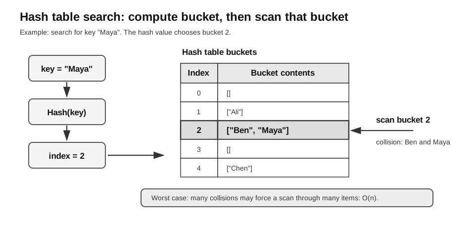
Caption: Follow the key through the hash function to one bucket, then scan only that bucket from left to right. This jump is valid because insertion and search use the same index rule; collided keys share the bucket and must still be compared individually.

Correctness invariant and preconditions: the table must contain at least one bucket, and every record must have been inserted using the same hash/index rule used by search. Therefore, if the key exists, it must be in the computed bucket. While scanning that bucket, every earlier record has already been ruled out by a failed key comparison.

Search contracts and duplicate behaviour: the shown linear search returns the first matching index encountered from left to right. The shown binary search may return any matching occurrence. The shown separate-chaining lookup returns the first matching record in its bucket. State a different contract explicitly if an application needs all matches or the first/last duplicate.

Implementation/Testing Bridge: Boundary-Test Matrix

This section connects the algorithms to the separate syllabus unit on validation, testing, and debugging. It is not an additional Unit 1.2 algorithm outcome.

Algorithm	Essential test cases	What the test protects against
linear search	empty list; singleton found/absent; target first/last; duplicates	missing absent return, wrong start/end bounds, unclear duplicate contract
binary search	empty list; singleton found/absent; target at each boundary; even/odd length; duplicates	skipped one-item range, incorrect midpoint or boundary update
hash-table search	empty bucket; collision bucket found/absent; key in first/last bucket	scanning wrong bucket, failing after a collision, out-of-range index

When debugging, trace the variables that define the remaining work: index for linear search, low/high/mid for binary search, and computed bucket plus current record for hash-table search.

Worked Debugging Example: A Range That Does Not Shrink

Suppose a faulty binary-search branch uses low <- mid when the target is larger. For [2, 5], target 5, the lower midpoint is repeatedly mid = 0: expected result is index 1, but the trace stays at low = 0, high = 1 forever. The first faulty state update is low <- mid, which leaves the range unchanged. Correct it to low <- mid + 1; a rerun gives low = high = mid = 1 and returns 1. Debugging means locating the first state that violates the progress invariant, not merely observing the final failure.

A Small Bucket Example

Suppose a keys-only teaching example has five buckets. It omits associated values to keep the collision trace simple; the executable version above stores (key, value) records.

Index	Bucket contents
0	[]
1	["Ali"]
2	["Ben", "Maya"]
3	[]
4	["Chen"]

If Hash("Maya") gives index 2, the search jumps directly to bucket 2 and checks ["Ben", "Maya"].

This is faster than scanning every stored name if the buckets are short.

However, "Ben" and "Maya" are in the same bucket. This is a collision. The algorithm still needs to search within that bucket.

Collision and Worst-Case Time

For worst-case Big-O comparison, hash table search can degrade to $O(n)$ if many keys collide and the algorithm must scan through a long bucket.

In a well-designed hash table, lookup is often very fast on average because the hash function spreads keys evenly. However, for this syllabus topic, the safest comparison is the worst case:

Situation	Search behaviour
keys spread evenly	check a short bucket
many keys collide	scan a long bucket
all keys collide into one bucket	may scan up to n items

The important idea is not the exact hash function. The important idea is that the key determines where to look. If the bucket contains several collided keys, the algorithm still has to search inside that bucket.

Good Hashing Algorithm Features

Exam questions may ask for features of a good hashing algorithm.

Feature	Why it matters
deterministic	the same key should always give the same hash value
fast to compute	lookup should not spend too much time calculating the position
spreads keys evenly	records should be distributed across the table, not clustered
minimises collisions	fewer keys share the same position or bucket
uses the table range	generated indexes should fit the available table positions

Do not say a good hash function has no collisions. Collisions are possible whenever many possible keys map into fewer table positions. A better answer is that it reduces collisions and has a collision-handling method.

Choosing a Search Algorithm

Situation	Suitable search method	Reason
unsorted small list	linear search	no ordering assumption is needed
unsorted list that is searched only once	linear search	sorting first may cost more effort than the search itself
sorted large list	binary search	each comparison discards about half the range
list is not sorted but many searches are needed	sort first, then consider binary search	sorting cost may be worthwhile if reused many times
key-value lookup, such as username to record	hash table search	the key can compute where to look
hash table with many collisions	may become slow	bucket search may approach linear search

A good answer should mention the data condition. For example, do not simply say “binary search is faster”. Say “binary search is faster for large sorted lists because it halves the search range each step”.

Comparing the Search Algorithms

Algorithm	Works on unsorted data?	Main state to trace	Worst-case time	Common trap
linear search	yes	index, item, comparison	$O(n)$	forgetting the absent case
binary search	no, data must be sorted	low, high, mid	$O(\log n)$	discarding halves on unsorted data
hash table search	data must be stored in a hash table	hash index, bucket	$O(n)$ worst case	claiming collisions cannot happen

How to Write Exam Explanations

Use precise cause-and-effect language.

Good explanation for linear search:

Linear search has worst-case time O(n) because the target may be last or absent, so the algorithm may need to compare the target with every item.

Good explanation for binary search:

Binary search has worst-case time O(log n) because the data is sorted and each comparison halves the remaining search range.

Good explanation for hash table search:

Hash table search uses a hash function to compute a bucket index. Its worst case is O(n) if many keys collide into the same bucket and the algorithm has to scan many items.

Avoid vague explanations such as:

• “Binary search is faster.”
• “Hashing is instant.”
• “Linear search is bad.”
• “A good hash function has no collisions.”

Common Mistakes

• Applying binary search to unsorted data.
• Forgetting to update low or high.
• Using while low < high when the algorithm still needs to check low == high.
• Setting low to mid or high to mid after mid has already been checked.
• Returning the item when the question asks for the index.
• Ignoring the absent-target case.
• Saying binary search is always better without considering whether the data is sorted.
• Saying a good hash function can guarantee no collisions for all possible keys.
• Treating hash table search as magic instead of linking it to hashing and collision handling.

Check Your Understanding

1. Linear search is run on [6, 3, 9, 1] with target 1. How many items are checked?
2. Linear search is run on [6, 3, 9, 1] with target 7. What value should be returned, and why?
3. Binary search is run on [2, 5, 8, 11, 14] with target 6. What are low, high, and mid after the first comparison?
4. Why is binary search invalid on [10, 4, 8, 2]?
5. In a binary search trace, what does low > high mean?
6. In hash table search, why can collisions make the worst case slower?
7. Why is it better to say that a hash function minimises collisions rather than prevents all collisions?
8. A list is unsorted and will be searched only once. Why might linear search be more suitable than sorting first and using binary search?

Related Notes

• Fundamental Algorithms
• Algorithm Efficiency and Tracing