Sorting Algorithms

Sorting rearranges data into order. The order may be ascending, descending, alphabetical, or based on a key field.

The syllabus sorting algorithms are:

• bubble sort;
• insertion sort;
• merge sort;
• quicksort.

A sorting algorithm is not just a piece of code that produces a sorted list. To understand a sorting algorithm properly, ask:

• What part of the list is already in a useful state?
• What comparison is made next?
• What values move, and why?
• What does one pass, insertion, merge, or partition achieve?
• What is the worst-case time complexity?

How to Trace Sorting Algorithms

A trace should show the important intermediate states, not only the final sorted list.

Different sorting algorithms need different trace units:

Algorithm	Main trace unit	What to record
bubble sort	pass	list after each pass; adjacent swaps during the pass if needed
insertion sort	insertion	current item, shifted items, list after insertion
merge sort	split and merge	sublists created during splitting; sorted lists produced during merging
quicksort	partition	pivot, less-than-pivot group, equal-to-pivot group, greater-than-pivot group

For beginner traces, it is better to show one small list carefully than to jump straight to a large example.

Bubble Sort

Bubble sort repeatedly compares adjacent items and swaps them if they are in the wrong order. After each full pass, a large item has moved towards the end of the list.

The key word is adjacent. Bubble sort does not search the whole list for the largest item and swap it directly. It moves large values step by step through neighbouring swaps.

Core Idea

For ascending order:

1. Compare the first pair of adjacent values.
2. Swap them if the left value is larger than the right value.
3. Move one position right and compare the next adjacent pair.
4. Continue until the end of the unsorted part is reached.
5. After one full pass, the largest value in the unsorted part has moved to its final position.

Original Python example:

def bubble_sort(values):
    values = values[:]
    n = len(values)
 
    for pass_number in range(n - 1):
        swapped = False
        for index in range(0, n - 1 - pass_number):
            if values[index] > values[index + 1]:
                values[index], values[index + 1] = values[index + 1], values[index]
                swapped = True
        if not swapped:
            break
 
    return values

The line values = values[:] makes a copy of the input list. This means the function returns a sorted copy instead of changing the original list supplied by the caller.

Language-Independent Pseudocode

FOR pass <- 0 TO LENGTH(values) - 2
    swapped <- FALSE
    FOR index <- 0 TO LENGTH(values) - 2 - pass
        IF values[index] > values[index + 1] THEN
            SWAP values[index], values[index + 1]
            swapped <- TRUE
        ENDIF
    NEXT index
    IF swapped = FALSE THEN RETURN values
NEXT pass
RETURN values

Invariant after pass p: the last p positions form a sorted suffix and contain the p largest values in their final positions. A non-optimised variant always performs the fixed passes; this optimised variant stops when a full pass makes no swap. The optimisation improves already-sorted behaviour but not the $O(n^2)$ worst case.

Trace for One Pass

Trace for one pass of [5, 2, 4, 1]:

Comparison	Action	List
5 and 2	swap	[2, 5, 4, 1]
5 and 4	swap	[2, 4, 5, 1]
5 and 1	swap	[2, 4, 1, 5]

After this pass, 5 is guaranteed to be in its final position at the end.

Full Pass-by-Pass Trace

For the same list [5, 2, 4, 1]:

Pass	Comparisons made in the unsorted part	List after pass	What is now fixed?
start	-	[5, 2, 4, 1]	nothing yet
1	compare up to the last position	[2, 4, 1, 5]	5 is fixed
2	ignore final 5; compare remaining part	[2, 1, 4, 5]	4, 5 are fixed
3	ignore final 4, 5; compare remaining part	[1, 2, 4, 5]	all values are fixed

The unsorted part becomes smaller after each pass because the largest remaining value has bubbled into its final position.

The swapped flag avoids unnecessary later passes when the list is already sorted.

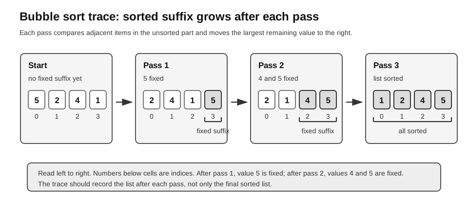
Caption: A bubble sort trace records the list after each pass and shows the fixed sorted suffix growing from the right.

Notice the pattern: after pass 1, the largest value 5 is at the end. After pass 2, 4 is in its final position. The unsorted part becomes smaller after each pass.

Bubble Sort Complexity

In the worst case, bubble sort needs repeated passes and many adjacent comparisons.

For a list of length $n$, the number of adjacent comparisons is roughly:

$$(n-1)+(n-2)+\cdots +2+1$$

This grows like $n^2$, so bubble sort has worst-case time complexity:

$$O(n^2)$$

An optimised bubble sort may stop early when no swaps occur in a pass. For an already sorted list, it can finish after one pass. However, the worst case remains $O(n^2)$.

Insertion Sort

Insertion sort builds a sorted section at the front of the list. Each new item from the unsorted section is inserted into the correct position in the sorted section.

This is similar to sorting a hand of playing cards: you take the next card and place it into the correct position among the cards already in order.

Core Idea

For ascending order:

1. Treat the first item as an already sorted section of length 1.
2. Take the next item as the current item.
3. Compare it with items in the sorted section from right to left.
4. Shift larger sorted items one position to the right.
5. Insert the current item into the opened position.
6. Repeat until all items have been inserted into the sorted section.

Original Python example:

def insertion_sort(values):
    values = values[:]
 
    for index in range(1, len(values)):
        current = values[index]
        position = index - 1
 
        while position >= 0 and values[position] > current:
            values[position + 1] = values[position]
            position = position - 1
 
        values[position + 1] = current
 
    return values

The variable current is important. It stores the item being inserted before larger items are shifted right. Without storing current, the value could be overwritten during shifting.

FOR index <- 1 TO LENGTH(values) - 1
    current <- values[index]
    position <- index - 1
    WHILE position >= 0 AND values[position] > current
        values[position + 1] <- values[position]
        position <- position - 1
    ENDWHILE
    values[position + 1] <- current
NEXT index

Invariant before each iteration: the prefix before index is sorted and contains exactly the same items that originally occupied that processed prefix.

Trace for One Insertion

Trace for inserting 2 into [5 | 2, 4, 1]:

Step	Sorted section idea	List
before insertion	[5] sorted, 2 current	[5, 2, 4, 1]
shift 5 right	space opens at index 0	[5, 5, 4, 1]
insert 2	[2, 5] sorted	[2, 5, 4, 1]

The temporary list [5, 5, 4, 1] is not an error. The original 2 has already been saved in current, so the algorithm can safely shift 5 right and later place 2 into the correct position.

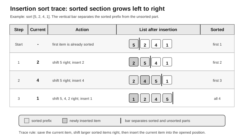
Caption: Insertion sort grows a sorted prefix by saving the current item, shifting larger sorted items right, and inserting the current item into the opened position.

When tracing insertion sort, keep asking: which part is already sorted, what is the current item, and which items must shift right to make space?

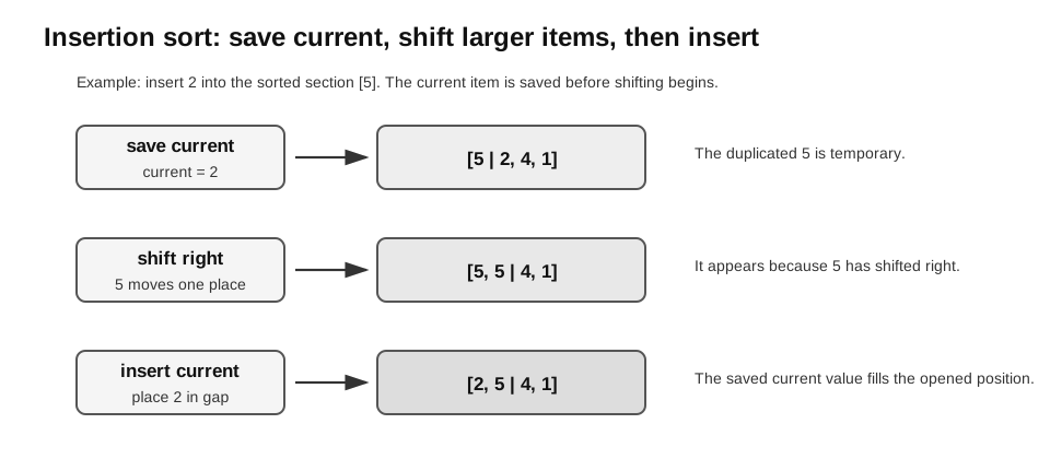
Caption: In insertion sort, larger items shift right first, then the current item is inserted into the opened position.

Full Insertion Trace

Trace for insertion sort on [5, 2, 4, 1]:

Pass	Current item	Shifts made	List after insertion	Sorted section after pass
start	-	-	[5, 2, 4, 1]	[5]
1	2	shift 5 right	[2, 5, 4, 1]	[2, 5]
2	4	shift 5 right	[2, 4, 5, 1]	[2, 4, 5]
3	1	shift 5, 4, 2 right	[1, 2, 4, 5]	[1, 2, 4, 5]

Insertion sort can be efficient on nearly sorted data because each current item may need only a small number of shifts.

Insertion Sort Complexity

In the worst case, each new item must move past many earlier items. This happens, for example, when sorting a descending list into ascending order.

The total number of shifts and comparisons grows like:

$$1+2+3+\cdots +(n-1)$$

Therefore, insertion sort has worst-case time complexity:

$$O(n^2)$$

Its best case can be much better when the list is already sorted, but the syllabus comparison here focuses on worst-case time complexity.

Merge Sort

Merge sort is a divide-and-conquer algorithm. It splits the list into smaller lists, sorts those smaller lists, then merges sorted lists back together.

The most important point is this: merge sort does most of its ordering work during the merge step, not during the split step.

Core Idea

1. If the list has length 0 or 1, it is already sorted.
2. Split the list into two halves.
3. Recursively apply merge sort to the left half.
4. Recursively apply merge sort to the right half.
5. Merge the two sorted halves into one sorted list.

A list of length 1 is considered sorted because there is no pair of items in the wrong order.

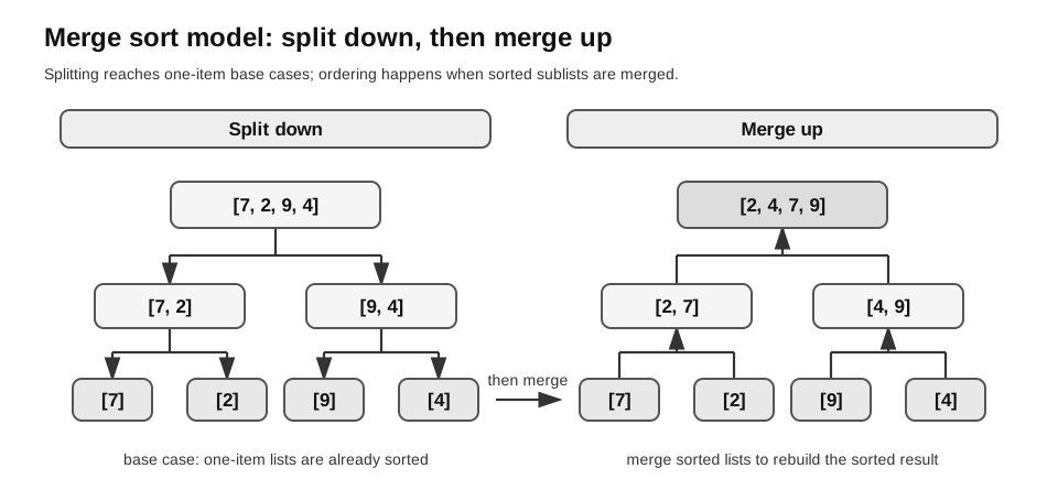
Caption: Merge sort splits down to one-item base cases, then does the ordering work while merging sorted sublists back up.

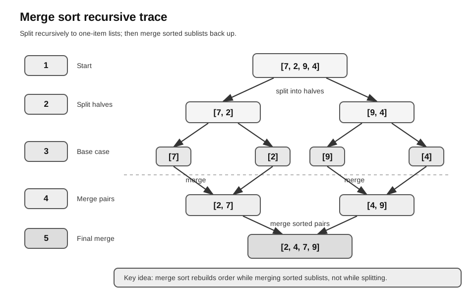
Caption: Read downward to follow recursive calls on strictly shorter sublists until each has length 1, then read upward to follow sorted merges. At every merge, compare the front unconsumed values and append the smaller one; when one side empties, append the other tail.

Original Python example:

def merge_sort(values):
    if len(values) <= 1:
        return values[:]
 
    mid = len(values) // 2
    left = merge_sort(values[:mid])
    right = merge_sort(values[mid:])
    return merge(left, right)
 
 
def merge(left, right):
    result = []
    left_index = 0
    right_index = 0
 
    while left_index < len(left) and right_index < len(right):
        if left[left_index] <= right[right_index]:
            result.append(left[left_index])
            left_index = left_index + 1
        else:
            result.append(right[right_index])
            right_index = right_index + 1
 
    result.extend(left[left_index:])
    result.extend(right[right_index:])
    return result

Language-independent structure:

FUNCTION MergeSort(values)
    IF LENGTH(values) <= 1 THEN RETURN COPY(values)
    mid <- LENGTH(values) DIV 2
    left <- MergeSort(values before mid)
    right <- MergeSort(values from mid onward)
    RETURN Merge(left, right)
ENDFUNCTION
 
FUNCTION Merge(left, right)
    result <- empty list
    i <- 0; j <- 0
    WHILE i < LENGTH(left) AND j < LENGTH(right)
        IF left[i] <= right[j] THEN
            APPEND left[i] TO result
            i <- i + 1
        ELSE
            APPEND right[j] TO result
            j <- j + 1
        ENDIF
    ENDWHILE
    APPEND every unconsumed item of left TO result
    APPEND every unconsumed item of right TO result
    RETURN result
ENDFUNCTION

During Merge, the output is always sorted and contains exactly the items already consumed from the two inputs; the unconsumed tails remain sorted. For an odd length, the lower-half split used here may be one item shorter, e.g. [5, 1, 4, 2, 3] splits into [5, 1] and [4, 2, 3]. Either side may receive the extra item if the convention is consistent.

Worked Merge Example

Suppose two smaller lists are already sorted:

left  = [2, 5]
right = [1, 4]

The merge process compares the front remaining items of the two lists:

Step	Compare	Append	Result so far	Remaining left	Remaining right
1	2 and 1	1	[1]	[2, 5]	[4]
2	2 and 4	2	[1, 2]	[5]	[4]
3	5 and 4	4	[1, 2, 4]	[5]	[]
4	right is empty	append remaining 5	[1, 2, 4, 5]	[]	[]

The merge step is efficient because it only moves forward through the two sorted lists.

Split-Down and Merge-Up Trace

For [5, 2, 4, 1]:

Split down:
[5, 2, 4, 1]
[5, 2]        [4, 1]
[5] [2]       [4] [1]
 
Merge up:
[5] + [2]  -> [2, 5]
[4] + [1]  -> [1, 4]
[2, 5] + [1, 4] -> [1, 2, 4, 5]

A common beginner mistake is to think splitting sorts the list. Splitting only breaks the problem into smaller parts. The sorted order is rebuilt during merging.

Merge Sort Complexity

Merge sort has worst-case time complexity:

$$O(n\log n)$$

Reason:

• the list is repeatedly halved, giving about $\log n$ levels;
• at each level, merging all sublists together takes about $n$ total work;
• therefore the total work is about $n\log n$.

Unlike quicksort, merge sort keeps splitting into halves in a predictable way, so its worst-case time remains $O(n\log n)$.

Quicksort

Quicksort chooses a pivot, partitions the list around the pivot, then recursively sorts the partitions.

Quicksort is also a divide-and-conquer algorithm, but it feels different from merge sort. Merge sort splits first and orders while merging. Quicksort partitions first, putting values on the correct side of the pivot before the recursive calls.

Core Idea

For the beginner-friendly out-of-place version:

1. If the list has length 0 or 1, it is already sorted.
2. Choose a pivot.
3. Put all values smaller than the pivot into less.
4. Put all values equal to the pivot into equal.
5. Put all values greater than the pivot into greater.
6. Recursively quicksort less and greater.
7. Return quicksort(less) + equal + quicksort(greater).

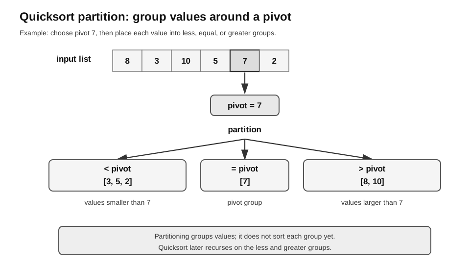
Caption: This figure explicitly chooses pivot 7. Follow each input value into exactly one of less, equal, or greater; the side groups satisfy their relation to 7 but are not yet internally sorted. The figure’s stated pivot is independent of the middle-index pivot rule used in the adjacent Python example.

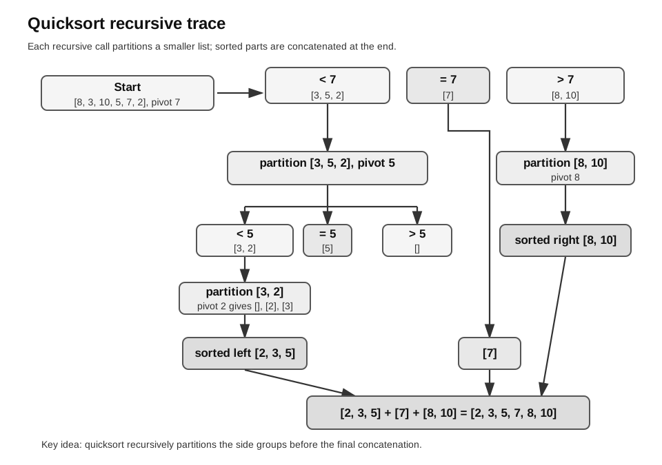
Caption: This trace starts with pivot 7, then uses the pivot stated at each child partition. Read downward through strictly smaller less and greater calls, then upward through concatenation. Values equal to a pivot are removed into equal, helping ensure the recursive side groups shrink even when duplicates occur.

Original out-of-place Python example:

def quicksort(values):
    if len(values) <= 1:
        return values[:]
 
    pivot = values[len(values) // 2]
    less = []
    equal = []
    greater = []
 
    for value in values:
        if value < pivot:
            less.append(value)
        elif value > pivot:
            greater.append(value)
        else:
            equal.append(value)
 
    return quicksort(less) + equal + quicksort(greater)

This version is easier to understand but not in-place because it creates new lists. In-place quicksort is an implementation refinement and can be treated later when implementation detail is the focus.

The code chooses the middle-index value as pivot. The two figures use independently stated pivots to make their traces spacious; they illustrate the same three-way partition rule but are not executions of this exact middle-pivot call. For any trace, write down the pivot rule or chosen pivot before partitioning.

FUNCTION QuickSort(values)
    IF LENGTH(values) <= 1 THEN RETURN COPY(values)
    pivot <- value at middle index
    less <- empty list; equal <- empty list; greater <- empty list
    FOR EACH value IN values
        IF value < pivot THEN
            APPEND value TO less
        ELSE IF value > pivot THEN
            APPEND value TO greater
        ELSE
            APPEND value TO equal
        ENDIF
    NEXT value
    RETURN QuickSort(less) + equal + QuickSort(greater)
ENDFUNCTION

Partition invariant: every original item occurs in exactly one group; all items in less are below the pivot, all in equal equal it, and all in greater exceed it. The groups less and greater need not yet be sorted. The equal group is essential for duplicates; for [3, 2, 3, 1, 3] with pivot 3, it becomes [3, 3, 3].

Recursive progress: merge sort calls itself on shorter halves until length 0 or 1. In this three-way quicksort, at least the pivot-equal item or items move into equal, so recursive less and greater calls are strictly shorter than the original list. If a recursive call receives an unchanged list, the partition or base case is faulty and termination is not guaranteed.

Worked Partition Example

For [5, 2, 4, 1], suppose the pivot is the middle item 4.

Value checked	Action	less	equal	greater
5	5 > 4, put in greater	[]	[]	[5]
2	2 < 4, put in less	[2]	[]	[5]
4	4 = 4, put in equal	[2]	[4]	[5]
1	1 < 4, put in less	[2, 1]	[4]	[5]

After this partition:

less    = [2, 1]
equal   = [4]
greater = [5]

This does not mean less is already sorted. It only means every value in less is smaller than the pivot. Quicksort must still sort less recursively.

The result will be:

quicksort([2, 1]) + [4] + quicksort([5])
= [1, 2] + [4] + [5]
= [1, 2, 4, 5]

Quicksort Complexity

Quicksort often performs well in practice when partitions are reasonably balanced.

If each pivot splits the list into two roughly equal parts, the behaviour is similar in shape to merge sort: about $\log n$ levels and about $n$ partitioning work per level. This gives about $O(n\log n)$ behaviour in good cases.

However, the syllabus worst-case time complexity is:

$$O(n^2)$$

The worst case occurs when pivot choices repeatedly create very unbalanced partitions, such as one empty partition and one almost-full partition.

For example, if a quicksort implementation always chooses the first item as pivot and the list is already sorted:

[1, 2, 3, 4, 5]

The pivot 1 gives:

less = []
equal = [1]
greater = [2, 3, 4, 5]

The next recursive call has almost the same problem again. This repeated imbalance leads to $O(n^2)$ worst-case time.

Choosing a Sorting Algorithm

Algorithm	Strength	Limitation
bubble sort	easy to trace	inefficient for large lists
insertion sort	good for small or nearly sorted lists	worst-case quadratic
merge sort	reliable $O(n\log n)$ worst case	uses extra lists in simple implementations
quicksort	often fast in practice	worst case depends on pivot balance

A useful beginner summary is:

Algorithm	Core method	Worst-case time	Good exam phrase
bubble sort	repeated adjacent swaps	$O(n^2)$	largest remaining value bubbles to the end after each pass
insertion sort	insert current item into sorted section	$O(n^2)$	sorted section grows from left to right
merge sort	split, sort, merge	$O(n\log n)$	ordering is rebuilt during merging
quicksort	pivot and partition	$O(n^2)$	bad pivots can create unbalanced partitions

For this syllabus topic, the main comparison is worst-case time complexity. Space complexity is not the core focus, although simple merge sort and out-of-place quicksort visibly create extra lists in their beginner-friendly implementations.

Implementation/Testing Bridge: Boundary Tests and Debugging

This section applies the separate testing/debugging syllabus outcomes to the four sorting implementations; it is not an extra sorting-algorithm requirement.

Run every sorting implementation on an empty list, a singleton, an already sorted list, a reverse-sorted list, and a list with duplicates. Also test an odd-length list for merge sort and an all-equal list for three-way quicksort. Check both that the result is ordered and that no item was lost or duplicated. A trace should record the algorithm’s own state: pass and suffix for bubble sort, sorted prefix for insertion sort, split/merge levels for merge sort, and pivot/groups for quicksort.

Common Mistakes

• Saying bubble sort swaps any two items; it swaps adjacent items.
• Forgetting that the largest remaining item is fixed after each bubble sort pass.
• Forgetting that insertion sort shifts items to make space.
• Thinking the temporary duplicated value during insertion sort shifting is an error.
• Describing merge sort as just splitting; the merge step is where ordering is rebuilt.
• Forgetting the base case in recursive sorting algorithms.
• Claiming quicksort always runs in $O(n\log n)$.
• Mixing up out-of-place and in-place quicksort.
• Treating quicksort partitioning as if each partition is already sorted.
• Not showing list states when asked to trace.

How to Write Exam Explanations

When explaining a sorting algorithm, use the algorithm’s key action.

For bubble sort:

Bubble sort repeatedly compares adjacent items and swaps them if they are in the wrong order. After each pass, the largest remaining item is moved to its final position.

For insertion sort:

Insertion sort keeps a sorted section at the front. It takes the next unsorted item, shifts larger sorted items right, and inserts the current item into the correct position.

For merge sort:

Merge sort recursively splits the list into smaller sublists until each has length 1, then merges sorted sublists to rebuild the final sorted list.

For quicksort:

Quicksort chooses a pivot, partitions values into less-than, equal-to, and greater-than groups, then recursively sorts the less and greater groups.

When explaining time complexity, include the reason, not only the Big-O result.

Good examples:

• Bubble sort is $O(n^2)$ in the worst case because it may need many passes with many adjacent comparisons.
• Insertion sort is $O(n^2)$ in the worst case because each current item may need to shift across many earlier items.
• Merge sort is $O(n\log n)$ because there are about $\log n$ split levels and each level requires about $n$ merge work.
• Quicksort is $O(n^2)$ in the worst case because bad pivot choices can repeatedly create highly unbalanced partitions.

Check Your Understanding

1. After one bubble sort pass on [4, 1, 3, 2], what value is guaranteed to be at the end?
2. In insertion sort, why do larger sorted items shift right before the current item is inserted?
3. Why is [5, 5, 4, 1] a reasonable temporary state when inserting 2 into [5, 2, 4, 1]?
4. In merge sort, why is a one-item list considered already sorted?
5. During merge sort, which step actually rebuilds the values in sorted order?
6. In quicksort, what does partitioning guarantee about values in less and greater?
7. In quicksort, why does an unbalanced partition lead to poor worst-case performance?
8. Why can an algorithm have a good best case but still have a worse worst-case Big-O?

Related Notes

• Fundamental Algorithms
• Algorithm Efficiency and Tracing