Algorithm Efficiency and Tracing
Tracing and efficiency answer different questions.
Tracing asks: what exactly happens on this input?
Efficiency asks: how does the amount of work grow as input size grows?
For this syllabus topic, both skills matter. A trace helps you show that you understand the algorithm step by step. A complexity explanation helps you compare algorithms when the input becomes larger.
The Main Idea
When studying an algorithm, do not jump straight to memorising its Big-O result.
A better learning sequence is:
- trace the algorithm on a small input;
- identify what work is repeated;
- ask how that repeated work changes when the input size becomes larger;
- express the growth using Big-O notation.
For example, if a linear search checks four items in a four-item list, then a larger list may require checking many more items. The exact number depends on the input, but the worst case grows in proportion to .
Tracing State Changes
When tracing an algorithm, record the variables that control the algorithm.
A good trace is not just the final answer. It should show enough intermediate states to prove how the algorithm reached that answer.
For linear search, useful trace columns are:
- index;
- current item;
- target comparison;
- return value if found.
For binary search, useful columns are:
- low;
- high;
- mid;
- middle value;
- action.
For sorting, useful traces depend on the algorithm:
| Algorithm | Useful trace unit | What to show |
|---|---|---|
| bubble sort | comparison and pass | adjacent comparisons, swaps, list after each pass |
| insertion sort | current item, shifting, insertion | sorted section, current item, shifted items, list after insertion |
| merge sort | split and merge result | how the list splits, then how sorted sublists merge |
| quicksort | pivot and partitions | pivot, less/equal/greater partitions, recursive results |
What Counts as a Step?
Big-O does not require counting exact machine instructions. At this level, a step usually means a meaningful unit of algorithmic work.
Examples of useful step ideas:
| Algorithm | Reasonable work to think about |
|---|---|
| linear search | checking one item against the target |
| binary search | one comparison with the middle item, followed by one range update |
| hash table search | computing a bucket, then checking items in that bucket if needed |
| bubble sort | one adjacent comparison, possibly followed by a swap |
| insertion sort | one comparison or one shift in the sorted section |
| merge sort | comparing front items while merging sorted sublists |
| quicksort | comparing each value with the pivot during partitioning |
The exact low-level operations are not the focus. The important question is how many repeated units of work may be needed as the input size grows.
Trace First, Then Generalise
Suppose linear search is run on:
[13, 8, 21, 5]If the target is 5, the algorithm checks all four items before finding it.
| Step | index | item | result |
|---|---|---|---|
| 1 | 0 | 13 | not found yet |
| 2 | 1 | 8 | not found yet |
| 3 | 2 | 21 | not found yet |
| 4 | 3 | 5 | found |
For this input, there are four checks.
Now generalise:
- with 10 items, the worst case may require 10 checks;
- with 100 items, the worst case may require 100 checks;
- with items, the worst case may require checks.
Therefore, the worst-case time complexity of linear search is .
This is the basic logic behind many complexity explanations: start from the trace, then describe how the trace would grow for larger inputs.
Big-O Notation
Big-O describes the growth of running time as input size n increases. For this syllabus topic, compare worst-case time complexity.
The exact number of machine instructions is not the focus. Big-O asks how the number of steps grows when the input grows.
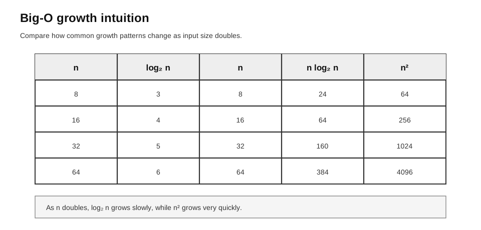
Caption: The table uses illustrative operation counts to compare growth functions, not benchmark timings. When input size doubles from 8 to 16, log₂ n increases only from 3 to 4, linear n doubles, and quadratic n² becomes four times as large. This is why repeated halving scales far better than quadratic work for large inputs, although Big-O alone does not predict exact seconds on a particular computer.
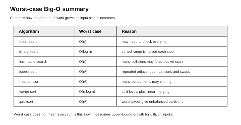
Caption: Read across each row from algorithm to worst-case Big-O and then to the causal explanation. The final column is essential: it distinguishes, for example, binary search’s repeated halving from quicksort’s possible sequence of unbalanced partitions, and prevents treating Big-O as an unexplained label.
Common growth patterns in this topic:
| Big-O | Meaning in this topic |
|---|---|
| constant time; not central for the main algorithms here | |
| repeated halving, such as binary search | |
| one pass through the input, such as linear search | |
| repeated splitting plus linear work per level, such as merge sort | |
| nested or repeated pairwise work, such as bubble sort worst case |
Growth Intuition with Small Numbers
The table below is not meant for exact timing. It helps you compare how quickly different growth patterns increase.
| 8 | 3 | 8 | 24 | 64 |
| 16 | 4 | 16 | 64 | 256 |
| 32 | 5 | 32 | 160 | 1024 |
| 64 | 6 | 64 | 384 | 4096 |
This is why repeated halving grows slowly, while quadratic algorithms become expensive quickly.
A common beginner mistake is to think and are similar because both look more complicated than . They are very different for large .
Worked Complexity Examples
Linear Search:
Linear search may need to check every item.
If the target is last or absent, the algorithm cannot stop early. For a list of length , up to items may be checked.
So the worst-case time complexity is .
Binary Search:
Binary search works on sorted data. Each comparison removes about half of the remaining search range.
For example, starting with 64 items:
64 -> 32 -> 16 -> 8 -> 4 -> 2 -> 1Only a small number of halvings is needed. The number of halvings grows logarithmically, so the worst-case time complexity is .
Bubble Sort:
Bubble sort repeatedly compares adjacent items across several passes.
In the worst case, the number of comparisons is approximately:
This sum grows quadratically with , so the worst-case time complexity is .
You do not need to memorise the exact sum formula for this topic, but you should understand the reason: many passes are made, and each pass may involve many comparisons.
Insertion Sort:
Insertion sort grows a sorted section. In the worst case, each new item must move past many earlier items.
For a reverse-sorted input, the first few insertions may shift:
1 item, then 2 items, then 3 items, and so onThis repeated shifting grows like in the worst case.
Merge Sort:
Merge sort repeatedly splits the list into halves, then merges sorted sublists.
There are about split levels. At each level, merging all sublists together involves about total work.
Therefore:
So the worst-case time complexity is .
Quicksort: Worst Case
Quicksort partitions values around a pivot. If the pivot repeatedly splits the data into two balanced parts, quicksort is usually efficient.
However, the syllabus comparison asks for worst case. In the worst case, the pivot repeatedly creates one empty or tiny partition and one almost-full partition.
For example, the sizes may shrink like this:
n, n - 1, n - 2, n - 3, ...That leads to quadratic growth, so quicksort’s worst-case time complexity is .
Worst Case Matters
Worst case means the input arrangement causes the algorithm to do the most work.
Examples:
- linear search: target is last or absent, so every item may be checked;
- binary search: target is not found until the range has been repeatedly halved;
- bubble sort: many adjacent swaps are needed;
- insertion sort: each new item may need to shift many earlier items;
- hash table search: many keys may collide into one bucket;
- quicksort: pivot choices repeatedly create highly unbalanced partitions.
Worst case is useful because it gives an upper-bound guarantee for comparison.
Best Case Is Not the Same
A best case can be much faster, but the syllabus comparison here focuses on worst case.
For example, linear search finds the target immediately if it is the first item. That does not change its worst-case time.
An optimised bubble sort may stop after one pass on an already sorted list. That is useful, but its worst case remains .
| Algorithm | Best-case idea | Worst-case idea | Syllabus comparison |
|---|---|---|---|
| linear search | target is first | target is last or absent | use worst-case |
| binary search | target is middle immediately | range must keep halving | use worst-case |
| optimised bubble sort | already sorted, no swaps after one pass | many swaps needed | use worst-case |
| insertion sort | already sorted or nearly sorted | reverse-sorted input causes many shifts | use worst-case |
| merge sort | still splits and merges | still splits and merges | use worst-case |
| quicksort | balanced partitions | highly unbalanced partitions | use worst-case |
Preconditions Affect Efficiency Comparisons
When comparing algorithms, always state any important precondition.
Binary search is only when the data is already sorted. If the data is unsorted, binary search is not valid.
A hash table search can be very fast in well-designed cases, but the worst case is still if many keys collide into the same bucket.
A complexity answer should not ignore these assumptions.
Complexity Summary
| Algorithm | Worst-case time | Reason |
|---|---|---|
| linear search | may check all n items | |
| binary search | halves the sorted search range | |
| hash table search | worst case | collisions may force a scan through many items |
| bubble sort | repeated adjacent comparisons and swaps | |
| insertion sort | repeated shifts in the sorted section | |
| merge sort | split levels plus merge work | |
| quicksort | worst pivot choices make unbalanced partitions |
How to Write Exam Explanations
A good answer should name the complexity and explain why.
Weak answer:
Linear search is O(n).Better answer:
Linear search has worst-case time complexity O(n) because the target may be at the last position or absent, so all n items may need to be checked.Useful sentence patterns:
| Situation | Sentence pattern |
|---|---|
| linear search | The worst case is because the algorithm may need to inspect every item. |
| binary search | The worst case is because each comparison halves the sorted search range. |
| bubble sort | The worst case is because the algorithm performs repeated adjacent comparisons over many passes. |
| insertion sort | The worst case is because each item may need to be compared with and shifted past many earlier items. |
| merge sort | The worst case is because there are about split levels and merging work per level. |
| quicksort | The worst case is because poor pivot choices can repeatedly create highly unbalanced partitions. |
Common Mistakes
- Counting only one loop iteration instead of considering input size.
- Comparing algorithms without stating the precondition, such as sorted data for binary search.
- Using best-case behaviour as if it were worst-case behaviour.
- Saying means the algorithm is always one step.
- Treating as the same as .
- Claiming quicksort is always .
- Saying hash table search is always without considering worst-case collisions.
- Discussing space complexity as if it were required core scope for this topic.
Check Your Understanding
- Why does linear search stay even though it may find the target at index 0?
- Why is binary search rather than ?
- Why does an optimised bubble sort still have worst-case time?
- Why is quicksort’s worst case worse than merge sort’s worst case?
- A binary search starts with 32 sorted items. Roughly how many times can the range be halved before only one item remains?
- Why is it not enough to say that an algorithm is fast on one small example?
- What precondition must be stated before comparing binary search with linear search?